Mathematical expectation of a random variable. Fundamentals of Probability Theory
2. Fundamentals of the theory of probability
Expected value
Consider a random variable with numerical values. It is often useful to associate a number with this function - its "mean value" or, as they say, "average value", "an indicator of the central tendency." For a number of reasons, some of which will become clear in what follows, it is common to use the mean as the mean.
Definition 3. Mathematical expectation of a random variable X called a number
those. the mathematical expectation of a random variable is a weighted sum of values of a random variable with weights equal to the probabilities of the corresponding elementary events.
Example 6 Let's calculate the mathematical expectation of the number that fell on the top face of the dice. It follows directly from Definition 3 that
Statement 2. Let the random variable X takes values x 1, x 2, ..., xm. Then the equality
![]() (5)
(5)
those. The mathematical expectation of a random variable is the weighted sum of the values of the random variable with weights equal to the probabilities that the random variable takes certain values.
In contrast to (4), where the summation is carried out directly over elementary events, a random event can consist of several elementary events.
Sometimes relation (5) is taken as the definition of the mathematical expectation. However, using Definition 3, as shown below, it is easier to establish the properties of the mathematical expectation needed to build probabilistic models of real phenomena than using relation (5).
To prove relation (5), we group in (4) terms with the same values of the random variable :

Since the constant factor can be taken out of the sign of the sum, then
By definition of the probability of an event
![]()
With the help of the last two relations, we obtain the desired:

The concept of mathematical expectation in probabilistic-statistical theory corresponds to the concept of the center of gravity in mechanics. Let's put it in the dots x 1, x 2, ..., xm on the numerical axis of the mass P(X= x 1 ), P(X= x 2 ),…, P(X= x m) respectively. Then equality (5) shows that the center of gravity of this system of material points coincides with the mathematical expectation, which shows the naturalness of Definition 3.
Statement 3. Let X- random value, M(X) is its mathematical expectation, A- some number. Then
1) M(a)=a; 2) M(X-M(X))=0; 3M[(X- a) 2 ]= M[(X- M(X)) 2 ]+(a- M(X)) 2 .
To prove this, we first consider a random variable that is constant, i.e. the function maps the space of elementary events to a single point A. Since the constant factor can be taken out of the sign of the sum, then
If each term of the sum is divided into two terms, then the whole sum is also divided into two sums, of which the first is made up of the first terms, and the second of the second. Therefore, the mathematical expectation of the sum of two random variables X+Y, defined on the same space of elementary events, is equal to the sum of mathematical expectations M(X) And M(U) these random variables:
M(X+Y) = M(X) + M(Y).
And therefore M(X-M(X)) = M(X) - M(M(X)). As shown above, M(M(X)) = M(X). Hence, M(X-M(X)) = M(X) - M(X) = 0.
Because the (X - a) 2 = ((X – M(X)) + (M(X) - a)} 2 = (X - M(X)) 2 + 2(X - M(X))(M(X) - a) + (M(X) – a) 2 , That M[(X - a) 2] =M(X - M(X)) 2 + M{2(X - M(X))(M(X) - a)} + M[(M(X) – a) 2 ]. Let's simplify the last equality. As shown at the beginning of the proof of Proposition 3, the expectation of a constant is the constant itself, and therefore M[(M(X) – a) 2 ] = (M(X) – a) 2 . Since the constant factor can be taken out of the sign of the sum, then M{2(X - M(X))(M(X) - a)} = 2(M(X) - a)M(X - M(X)). The right hand side of the last equality is 0 because, as shown above, M(X-M(X))=0. Hence, M[(X- a) 2 ]= M[(X- M(X)) 2 ]+(a- M(X)) 2 , which was to be proved.
From what has been said, it follows that M[(X- a) 2 ] reaches a minimum A equal to M[(X- M(X)) 2 ], at a = M(X), since the second term in equality 3) is always non-negative and equals 0 only for the specified value A.
Statement 4. Let the random variable X takes values x 1, x 2, ..., xm, and f is some function of a numeric argument. Then
![]()
To prove it, let's group on the right side of equality (4), which determines the mathematical expectation, terms with the same values:

Using the fact that the constant factor can be taken out of the sign of the sum, and by determining the probability of a random event (2), we obtain
Q.E.D.
Statement 5. Let X And At are random variables defined on the same space of elementary events, A And b- some numbers. Then M(aX+ bY)= aM(X)+ bM(Y).
Using the definition of the mathematical expectation and the properties of the summation symbol, we obtain a chain of equalities:

The required is proved.
The above shows how the mathematical expectation depends on the transition to another origin and to another unit of measurement (transition Y=aX+b), as well as to functions of random variables. The results obtained are constantly used in technical and economic analysis, in assessing the financial and economic activities of an enterprise, in the transition from one currency to another in foreign economic settlements, in regulatory and technical documentation, etc. The considered results allow using the same calculation formulas for various parameters scale and shift.
| Previous |
The mathematical expectation of a discrete random variable is the sum of the products of all its possible values and their probabilities.
Let a random variable can take only the probabilities of which are respectively equal. Then the mathematical expectation of a random variable is determined by the equality
If a discrete random variable takes on a countable set of possible values, then
Moreover, the mathematical expectation exists if the series on the right side of the equality converges absolutely.
Comment. It follows from the definition that the mathematical expectation of a discrete random variable is a non-random (constant) variable.
Definition of mathematical expectation in the general case
Let us define the mathematical expectation of a random variable whose distribution is not necessarily discrete. Let's start with the case of non-negative random variables. The idea will be to approximate such random variables with the help of discrete ones, for which the mathematical expectation has already been determined, and set the mathematical expectation equal to the limit of mathematical expectations of the discrete random variables approximating it. By the way, this is a very useful general idea, which consists in the fact that some characteristic is first determined for simple objects, and then for more complex objects it is determined by approximating them with simpler ones.
Lemma 1. Let there be an arbitrary non-negative random variable. Then there is a sequence of discrete random variables such that

Proof. Let us divide the semiaxis into equal segments of length and define
Then properties 1 and 2 follow easily from the definition of a random variable, and
Lemma 2. Let be a non-negative random variable and and two sequences of discrete random variables with properties 1-3 from Lemma 1. Then
Proof. Note that for non-negative random variables we allow
By property 3, it is easy to see that there is a sequence of positive numbers such that
Hence it follows that
Using the properties of mathematical expectations for discrete random variables, we obtain
Passing to the limit as we obtain the assertion of Lemma 2.
Definition 1. Let be a non-negative random variable, be a sequence of discrete random variables with properties 1-3 from Lemma 1. The mathematical expectation of a random variable is the number
Lemma 2 guarantees that it does not depend on the choice of the approximating sequence.
Let now be an arbitrary random variable. Let's define


From the definition and it easily follows that

Definition 2. The mathematical expectation of an arbitrary random variable is the number
If at least one of the numbers on the right side of this equality is finite.
Expectation Properties
Property 1. The mathematical expectation of a constant value is equal to the constant itself:
Proof. We will consider the constant as a discrete random variable that has one possible value and takes it with probability, therefore,
Remark 1. We define the product of a constant value by a discrete random variable as a discrete random variable whose possible values are equal to the products of a constant by possible values; the probabilities of possible values are equal to the probabilities of the corresponding possible values. For example, if the probability of a possible value is equal, then the probability that the value will take on a value is also equal to
Property 2. A constant factor can be taken out of the expectation sign:
Proof. Let the random variable be given by the probability distribution law:
Considering Remark 1, we write the law of distribution of the random variable
Remark 2. Before proceeding to the next property, we indicate that two random variables are called independent if the distribution law of one of them does not depend on what possible values the other variable has taken. Otherwise, the random variables are dependent. Several random variables are called mutually independent if the laws of distribution of any number of them do not depend on what possible values the other variables have taken.
Remark 3. We define the product of independent random variables and as a random variable the possible values of which are equal to the products of each possible value by each possible value of the probabilities of the possible values of the product are equal to the products of the probabilities of the possible values of the factors. For example, if the probability of a possible value is, the probability of a possible value is then the probability of a possible value is
Property 3. The mathematical expectation of the product of two independent random variables is equal to the product of their mathematical expectations:
Proof. Let independent random variables and be given by their own probability distribution laws:
Let's make up all the values that a random variable can take. To do this, we multiply all possible values by each possible value; as a result, we obtain and, taking into account Remark 3, we write the distribution law assuming for simplicity that all possible values of the product are different (if this is not the case, then the proof is carried out similarly):
The mathematical expectation is equal to the sum of the products of all possible values and their probabilities:
Consequence. The mathematical expectation of the product of several mutually independent random variables is equal to the product of their mathematical expectations.
Property 4. The mathematical expectation of the sum of two random variables is equal to the sum of the mathematical expectations of the terms:
Proof. Let random variables and be given by the following distribution laws:
Compose all possible values of the quantity To do this, add each possible value to each possible value; we obtain Suppose for simplicity that these possible values are different (if this is not the case, then the proof is carried out in a similar way), and we denote their probabilities by and respectively
The mathematical expectation of a value is equal to the sum of the products of possible values by their probabilities:
Let us prove that an Event consisting in taking a value (the probability of this event is equal) entails an event that consists in taking the value or (the probability of this event is equal by the addition theorem), and vice versa. Hence it follows that The equalities
Substituting the right parts of these equalities into relation (*), we obtain
or finally
Dispersion and standard deviation
In practice, it is often required to estimate the dispersion of possible values of a random variable around its mean value. For example, in artillery it is important to know how closely the shells will fall close to the target that should be hit.
At first glance, it may seem that the easiest way to estimate the scattering is to calculate all possible values of the deviation of a random variable and then find their average value. However, this path will not give anything, since the average value of the deviation, i.e. for any random variable is zero. This property is explained by the fact that some possible deviations are positive, while others are negative; as a result of their mutual cancellation, the average value of the deviation is zero. These considerations indicate the expediency of replacing possible deviations with their absolute values or their squares. That is how they do it in practice. True, in the case when possible deviations are replaced by their absolute values, one has to operate with absolute values, which sometimes leads to serious difficulties. Therefore, most often they go the other way, i.e. calculate the average value of the squared deviation, which is called the variance.
There will also be tasks for an independent solution, to which you can see the answers.
Mathematical expectation and variance are the most commonly used numerical characteristics of a random variable. They characterize the most important features of the distribution: its position and degree of dispersion. The mathematical expectation is often referred to simply as the mean. random variable. Dispersion of a random variable - a characteristic of dispersion, dispersion of a random variable around its mathematical expectation.
In many problems of practice, a complete, exhaustive description of a random variable - the law of distribution - either cannot be obtained, or is not needed at all. In these cases, they are limited to an approximate description of a random variable using numerical characteristics.
Mathematical expectation of a discrete random variable
Let's come to the concept of mathematical expectation. Let the mass of some substance be distributed between the points of the x-axis x1 , x 2 , ..., x n. Moreover, each material point has a mass corresponding to it with a probability of p1 , p 2 , ..., p n. It is required to select one point on the x-axis, which characterizes the position of the entire system of material points, taking into account their masses. It is natural to take the center of mass of the system of material points as such a point. This is the weighted average of the random variable X, in which the abscissa of each point xi enters with a "weight" equal to the corresponding probability. The mean value of the random variable thus obtained X is called its mathematical expectation.
The mathematical expectation of a discrete random variable is the sum of the products of all its possible values and the probabilities of these values:
Example 1 A win-win lottery was organized. There are 1000 winnings, 400 of which are 10 rubles each. 300 - 20 rubles each 200 - 100 rubles each. and 100 - 200 rubles each. What is the average winnings for a person who buys one ticket?
Solution. We will find the average win if the total amount of winnings, which is equal to 10*400 + 20*300 + 100*200 + 200*100 = 50,000 rubles, is divided by 1000 (the total amount of winnings). Then we get 50000/1000 = 50 rubles. But the expression for calculating the average gain can also be represented in the following form:
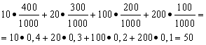
On the other hand, under these conditions, the amount of winnings is a random variable that can take on the values of 10, 20, 100 and 200 rubles. with probabilities equal to 0.4, respectively; 0.3; 0.2; 0.1. Therefore, the expected average payoff is equal to the sum of the products of the size of the payoffs and the probability of receiving them.
Example 2 The publisher decided to publish a new book. He is going to sell the book for 280 rubles, of which 200 will be given to him, 50 to the bookstore, and 30 to the author. The table gives information about the cost of publishing a book and the likelihood of selling a certain number of copies of the book.
Find the publisher's expected profit.
Solution. The random variable "profit" is equal to the difference between the income from the sale and the cost of the costs. For example, if 500 copies of a book are sold, then the income from the sale is 200 * 500 = 100,000, and the cost of publishing is 225,000 rubles. Thus, the publisher faces a loss of 125,000 rubles. The following table summarizes the expected values of the random variable - profit:
| Number | Profit xi | Probability pi | xi p i |
| 500 | -125000 | 0,20 | -25000 |
| 1000 | -50000 | 0,40 | -20000 |
| 2000 | 100000 | 0,25 | 25000 |
| 3000 | 250000 | 0,10 | 25000 |
| 4000 | 400000 | 0,05 | 20000 |
| Total: | 1,00 | 25000 |
Thus, we obtain the mathematical expectation of the publisher's profit:
![]() .
.
Example 3 Chance to hit with one shot p= 0.2. Determine the consumption of shells that provide the mathematical expectation of the number of hits equal to 5.
Solution. From the same expectation formula that we have used so far, we express x- consumption of shells:
![]() .
.
Example 4 Determine the mathematical expectation of a random variable x number of hits with three shots, if the probability of hitting with each shot p = 0,4 .
Hint: find the probability of the values of a random variable by Bernoulli formula .
Expectation Properties
Consider the properties of mathematical expectation.
Property 1. The mathematical expectation of a constant value is equal to this constant:
Property 2. The constant factor can be taken out of the expectation sign:
Property 3. The mathematical expectation of the sum (difference) of random variables is equal to the sum (difference) of their mathematical expectations:
Property 4. The mathematical expectation of the product of random variables is equal to the product of their mathematical expectations:
Property 5. If all values of the random variable X decrease (increase) by the same number WITH, then its mathematical expectation will decrease (increase) by the same number:
![]()
When you can not be limited only to mathematical expectation
In most cases, only the mathematical expectation cannot adequately characterize a random variable.
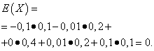
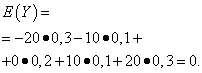
Let random variables X And Y are given by the following distribution laws:
| Meaning X | Probability |
| -0,1 | 0,1 |
| -0,01 | 0,2 |
| 0 | 0,4 |
| 0,01 | 0,2 |
| 0,1 | 0,1 |
| Meaning Y | Probability |
| -20 | 0,3 |
| -10 | 0,1 |
| 0 | 0,2 |
| 10 | 0,1 |
| 20 | 0,3 |
The mathematical expectations of these quantities are the same - equal to zero:
However, their distribution is different. Random value X can only take values that are little different from the mathematical expectation, and the random variable Y can take values that deviate significantly from the mathematical expectation. A similar example: the average wage does not make it possible to judge the proportion of high- and low-paid workers. In other words, by mathematical expectation one cannot judge what deviations from it, at least on average, are possible. To do this, you need to find the variance of a random variable.
Dispersion of a discrete random variable
dispersion discrete random variable X is called the mathematical expectation of the square of its deviation from the mathematical expectation:
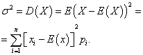
The standard deviation of a random variable X is the arithmetic value of the square root of its variance:
![]() .
.
Example 5 Calculate variances and standard deviations of random variables X And Y, whose distribution laws are given in the tables above.
Solution. Mathematical expectations of random variables X And Y, as found above, are equal to zero. According to the dispersion formula for E(X)=E(y)=0 we get:
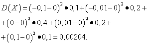
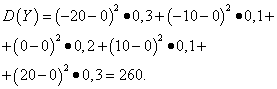
Then the standard deviations of random variables X And Y constitute
![]() .
.
Thus, with the same mathematical expectations, the variance of the random variable X very small and random Y- significant. This is a consequence of the difference in their distribution.
Example 6 The investor has 4 alternative investment projects. The table summarizes the data on the expected profit in these projects with the corresponding probability.
| Project 1 | Project 2 | Project 3 | Project 4 |
| 500, P=1 | 1000, P=0,5 | 500, P=0,5 | 500, P=0,5 |
| 0, P=0,5 | 1000, P=0,25 | 10500, P=0,25 | |
| 0, P=0,25 | 9500, P=0,25 |
Find for each alternative the mathematical expectation, variance and standard deviation.
Solution. Let us show how these quantities are calculated for the 3rd alternative:
The table summarizes the found values for all alternatives.
All alternatives have the same mathematical expectation. This means that in the long run everyone has the same income. The standard deviation can be interpreted as a measure of risk - the larger it is, the greater the risk of the investment. An investor who doesn't want much risk will choose project 1 because it has the smallest standard deviation (0). If the investor prefers risk and high returns in a short period, then he will choose the project with the largest standard deviation - project 4.
Dispersion Properties
Let us present the properties of the dispersion.
Property 1. The dispersion of a constant value is zero:
Property 2. The constant factor can be taken out of the dispersion sign by squaring it:
![]() .
.
Property 3. The variance of a random variable is equal to the mathematical expectation of the square of this value, from which the square of the mathematical expectation of the value itself is subtracted:
![]() ,
,
Where ![]() .
.
Property 4. The variance of the sum (difference) of random variables is equal to the sum (difference) of their variances:
Example 7 It is known that a discrete random variable X takes only two values: −3 and 7. In addition, the mathematical expectation is known: E(X) = 4 . Find the variance of a discrete random variable.
Solution. Denote by p the probability with which a random variable takes on a value x1 = −3 . Then the probability of the value x2 = 7 will be 1 − p. Let's derive the equation for mathematical expectation:
E(X) = x 1 p + x 2 (1 − p) = −3p + 7(1 − p) = 4 ,
where we get the probabilities: p= 0.3 and 1 − p = 0,7 .
The law of distribution of a random variable:
| X | −3 | 7 |
| p | 0,3 | 0,7 |
We calculate the variance of this random variable using the formula from property 3 of the variance:
D(X) = 2,7 + 34,3 − 16 = 21 .
Find the mathematical expectation of a random variable yourself, and then see the solution
Example 8 Discrete random variable X takes only two values. It takes the larger value of 3 with a probability of 0.4. In addition, the variance of the random variable is known D(X) = 6 . Find the mathematical expectation of a random variable.
Example 9 An urn contains 6 white and 4 black balls. 3 balls are taken from the urn. The number of white balls among the drawn balls is a discrete random variable X. Find the mathematical expectation and variance of this random variable.
Solution. Random value X can take the values 0, 1, 2, 3. The corresponding probabilities can be calculated from rule of multiplication of probabilities. The law of distribution of a random variable:
| X | 0 | 1 | 2 | 3 |
| p | 1/30 | 3/10 | 1/2 | 1/6 |
Hence the mathematical expectation of this random variable:
M(X) = 3/10 + 1 + 1/2 = 1,8 .
The variance of a given random variable is:
D(X) = 0,3 + 2 + 1,5 − 3,24 = 0,56 .
Mathematical expectation and dispersion of a continuous random variable
For a continuous random variable, the mechanical interpretation of the mathematical expectation will retain the same meaning: the center of mass for a unit mass distributed continuously on the x-axis with density f(x). In contrast to a discrete random variable, for which the function argument xi changes abruptly, for a continuous random variable, the argument changes continuously. But the mathematical expectation of a continuous random variable is also related to its mean value.
To find the mathematical expectation and variance of a continuous random variable, you need to find definite integrals . If a density function of a continuous random variable is given, then it enters directly into the integrand. If a probability distribution function is given, then by differentiating it, you need to find the density function.
The arithmetic average of all possible values of a continuous random variable is called its mathematical expectation, denoted by or .
Solution:
6.1.2 Expectation Properties
1. The mathematical expectation of a constant value is equal to the constant itself.
2. A constant factor can be taken out of the expectation sign. ![]()
3. The mathematical expectation of the product of two independent random variables is equal to the product of their mathematical expectations.
This property is valid for an arbitrary number of random variables.
4. The mathematical expectation of the sum of two random variables is equal to the sum of the mathematical expectations of the terms.
This property is also true for an arbitrary number of random variables.
Example: M(X) = 5, M(Y)= 2. Find the mathematical expectation of a random variable Z, applying the properties of mathematical expectation, if it is known that Z=2X + 3Y.
Solution: M(Z) = M(2X + 3Y) = M(2X) + M(3Y) = 2M(X) + 3M(Y) = 2∙5+3∙2 =
1) the mathematical expectation of the sum is equal to the sum of the mathematical expectations
2) the constant factor can be taken out of the expectation sign
Let n independent trials be performed, the probability of occurrence of event A in which is equal to p. Then the following theorem holds:
Theorem. The mathematical expectation M(X) of the number of occurrences of event A in n independent trials is equal to the product of the number of trials and the probability of occurrence of the event in each trial.
6.1.3 Dispersion of a discrete random variable
Mathematical expectation cannot fully characterize a random process. In addition to the mathematical expectation, it is necessary to introduce a value that characterizes the deviation of the values of the random variable from the mathematical expectation.
This deviation is equal to the difference between the random variable and its mathematical expectation. In this case, the mathematical expectation of the deviation is zero. This is explained by the fact that some possible deviations are positive, others are negative, and as a result of their mutual cancellation, zero is obtained.
Dispersion (scattering) Discrete random variable is called the mathematical expectation of the squared deviation of the random variable from its mathematical expectation.
In practice, this method of calculating the variance is inconvenient, because leads to cumbersome calculations for a large number of values of a random variable.
Therefore, another method is used.
Theorem. The variance is equal to the difference between the mathematical expectation of the square of the random variable X and the square of its mathematical expectation.
Proof. Taking into account the fact that the mathematical expectation M (X) and the square of the mathematical expectation M 2 (X) are constant values, we can write:
Example. Find the variance of a discrete random variable given by the distribution law.
| X | ||||
| X 2 | ||||
| R | 0.2 | 0.3 | 0.1 | 0.4 |
Solution: .
6.1.4 Dispersion properties
1. The dispersion of a constant value is zero. .
2. A constant factor can be taken out of the dispersion sign by squaring it. ![]() .
.
3. The variance of the sum of two independent random variables is equal to the sum of the variances of these variables. .
4. The variance of the difference of two independent random variables is equal to the sum of the variances of these variables. .
Theorem. The variance of the number of occurrences of event A in n independent trials, in each of which the probability p of the occurrence of the event is constant, is equal to the product of the number of trials and the probability of occurrence and non-occurrence of the event in each trial.
Example: Find the variance of DSV X - the number of occurrences of event A in 2 independent trials, if the probability of occurrence of the event in these trials is the same and it is known that M(X) = 1.2.
We apply the theorem from Section 6.1.2:
M(X) = np
M(X) = 1,2; n= 2. Find p:
1,2 = 2∙p
p = 1,2/2
q = 1 – p = 1 – 0,6 = 0,4
Let's find the dispersion by the formula:
D(X) = 2∙0,6∙0,4 = 0,48
6.1.5 Standard deviation of a discrete random variable
Standard deviation random variable X is called the square root of the variance.
![]() (25)
(25)
Theorem. The standard deviation of the sum of a finite number of mutually independent random variables is equal to the square root of the sum of the squared standard deviations of these variables.
6.1.6 Mode and median of a discrete random variable
Fashion M o DSV the most probable value of a random variable is called (i.e. the value that has the highest probability)
Median M e DSV is the value of a random variable that divides the distribution series in half. If the number of values of the random variable is even, then the median is found as the arithmetic mean of the two mean values.
Example: Find Mode and Median of DSW X:
| X | ||||
| p | 0.2 | 0.3 | 0.1 | 0.4 |
Me = = 5,5
Progress
1. Get acquainted with the theoretical part of this work (lectures, textbook).
2. Complete the task according to your choice.
3. Compile a report on the work.
4. Protect your work.
2. The purpose of the work.
3. Progress of work.
4. Decision of your option.
6.4 Variants of tasks for independent work
Option number 1
1. Find the mathematical expectation, variance, standard deviation, mode and median of DSV X given by the distribution law.
| X | ||||
| P | 0.1 | 0.6 | 0.2 | 0.1 |
2. Find the mathematical expectation of a random variable Z, if the mathematical expectations of X and Y are known: M(X)=6, M(Y)=4, Z=5X+3Y.
3. Find the variance of DSV X - the number of occurrences of event A in two independent trials, if the probabilities of occurrence of events in these trials are the same and it is known that M (X) = 1.
4. A list of possible values of a discrete random variable is given X: x 1 = 1, x2 = 2, x 3= 5, and the mathematical expectations of this quantity and its square are also known: , . Find the probabilities , , , corresponding to the possible values , , and draw up the distribution law of the DSV.
Option number 2
| X | ||||
| P | 0.3 | 0.1 | 0.2 | 0.4 |
2. Find the mathematical expectation of a random variable Z if the mathematical expectations of X and Y are known: M(X)=5, M(Y)=8, Z=6X+2Y.
3. Find the variance of DSV X - the number of occurrences of event A in three independent trials, if the probabilities of occurrence of events in these trials are the same and it is known that M (X) = 0.9.
4. A list of possible values of a discrete random variable X is given: x 1 = 1, x2 = 2, x 3 = 4, x4= 10, and the mathematical expectations of this quantity and its square are also known: , . Find the probabilities , , , corresponding to the possible values , , and draw up the distribution law of the DSV.
Option number 3
1. Find the mathematical expectation, variance and standard deviation of the DSV X given by the distribution law.
| X | ||||
| P | 0.5 | 0.1 | 0.2 | 0.3 |
2. Find the mathematical expectation of a random variable Z, if the mathematical expectations of X and Y are known: M(X)=3, M(Y)=4, Z=4X+2Y.
3. Find the variance of DSV X - the number of occurrences of event A in four independent trials, if the probabilities of occurrence of events in these trials are the same and it is known that M (x) = 1.2.
As already known, the distribution law completely characterizes a random variable. However, the distribution law is often unknown and one has to limit oneself to lesser information. Sometimes it is even more profitable to use numbers that describe a random variable in total; such numbers are called numerical characteristics of a random variable.
Mathematical expectation is one of the important numerical characteristics.
The mathematical expectation is approximately equal to the average value of a random variable.
Mathematical expectation of a discrete random variable is the sum of the products of all its possible values and their probabilities.
If a random variable is characterized by a finite distribution series:
| X | x 1 | x 2 | x 3 | … | x n |
| R | p 1 | p 2 | p 3 | … | r p |
then the mathematical expectation M(X) is determined by the formula:
The mathematical expectation of a continuous random variable is determined by the equality:
where is the probability density of the random variable X.
Example 4.7. Find the mathematical expectation of the number of points that fall out when a dice is thrown.
Solution:
Random value X takes the values 1, 2, 3, 4, 5, 6. Let's make the law of its distribution:
| X | ||||||
| R |
Then the mathematical expectation is:
Properties of mathematical expectation:
1. The mathematical expectation of a constant value is equal to the constant itself:
M(S)=S.
2. The constant factor can be taken out of the expectation sign:
M(CX) = CM(X).
3. The mathematical expectation of the product of two independent random variables is equal to the product of their mathematical expectations:
M(XY) = M(X)M(Y).
Example 4.8. Independent random variables X And Y are given by the following distribution laws:
| X | Y | ||||||
| R | 0,6 | 0,1 | 0,3 | R | 0,8 | 0,2 |
Find the mathematical expectation of a random variable XY.
Solution.
Let's find the mathematical expectations of each of these quantities:
random variables X And Y independent, so the desired mathematical expectation:
M(XY) = M(X)M(Y)=
Consequence. The mathematical expectation of the product of several mutually independent random variables is equal to the product of their mathematical expectations.
4. The mathematical expectation of the sum of two random variables is equal to the sum of the mathematical expectations of the terms:
M(X + Y) = M(X) + M(Y).
Consequence. The mathematical expectation of the sum of several random variables is equal to the sum of the mathematical expectations of the terms.
Example 4.9. 3 shots are fired with probabilities of hitting the target equal to p 1 = 0,4; p2= 0.3 and p 3= 0.6. Find the mathematical expectation of the total number of hits.
Solution.
The number of hits on the first shot is a random variable X 1, which can take only two values: 1 (hit) with probability p 1= 0.4 and 0 (miss) with probability q 1 = 1 – 0,4 = 0,6.
The mathematical expectation of the number of hits in the first shot is equal to the probability of hitting:
Similarly, we find the mathematical expectations of the number of hits in the second and third shots:
M(X 2)= 0.3 and M (X 3) \u003d 0,6.
The total number of hits is also a random variable consisting of the sum of hits in each of the three shots:
X \u003d X 1 + X 2 + X 3.
The desired mathematical expectation X we find by the theorem of mathematical, the expectation of the sum.


